Monday, August 30, 2010

TempLS V2 Math basis

The Math basis of TempLS Ver 2

For Version 1 of TempLS I posted a PDF guide, TempLS.pdf, to the mathematical basis. It's a useful starting point here.

But this time I'm going to try to do it in HTML below. Colors help.

For more Version 2 information:


  • Index of posts by category
  • TempLS Version 2 Release
  • Ver 2 - Regional spatial variation.
  • Spatial Temperature distributions in TempLS V2
  • Plotting spatial trends in TempLS


  •  Notation

    I need to use a summation convention. I'm referring to various matrices etc as just indexed sets, and when they are multiplied together, every index that appears twice is understood to be summed over the range of that index. It's called a dummy index, because it doesn't matter what symbol you use (as long as it's not used for something else). Once the summation is done, that index doesn't connect with anything else.

    I'll be talking about weighted least squares, and an exception is needed for the weight function. It's indices are sometimes put in brackets, which means they should not be counted in this pairing. The index still varies with any summation that is going on.

    The reason for this is that summation signs are difficult in HTML. But also it gets easier with colors. I'll color indices subject to summation blue, standalone indices red, and exception indices lime green.

    So multiplying two matrices A and B (C=A*B) would be represented:
    Cik  =  Aij Bjk

    The model

    We have, on the GHCN and similar sets, a number of stations (s), with temperature readings (x) by year (y) and month (m). m varies 1:12. The model is that x can be represented by a local temperature L, with a value for each station and month (seasonal average), and a global temperature G depending on year alone.

    xsmy  ~  Lsm  +  Gy
    It's useful to maintain a convention that every term has to include every red index. So I'll introduce an identity Iy, for which every component is 1, and rewrite the model as
    xsmy  ~  IyLsm  +  IsmGy

    Weighted least squares.

    The L and G are parameters to be fitted. We minimise a weighted squares expression for the residuals. The weight function w has two important roles.
    • It is zero for missing values
    • It needs to ensure that stations make "fair" contributions to the sum, so that regions with many stations aren't over-represented. This means that the sum with weights should be like a numerical integral over the surface. w should be inversely proportional to station density.
    So we want to minimise w(smy)(xsmy - IyLsm - IsmGy)2

    Differentiation

    This is done by differentiating this expression wrt each parameter component. In the summation convention, when you differentiate wrt a paired index, it disappears. The remaining index goes from blue to red. The original scalar SS becomes a system of equations, as the red indices indicate:
    Minimise:w(smy)(xsmy - IyLsm - IsmGy)2
    Differentiate wrt L:   w(smy)Iy(xsmy - IyLsm - IsmGy) = 0
    Differentiate wrt G:w(smy)Ism(xsmy - IyLsm - IsmGy) = 0


    The identity operations have been useful, but can now be rationalised. The equations become:

    Differentiate wrt L:   w(sm)y IyLsm  +  wsmy Gy  =  w(sm)y xsmy
    Differentiate wrt G:wsmy Lsm  +  wsm(y) IsmGy  =  wsm(y) xsmy

    Equations to be solved

    These are the equations to be solved for L and G. It can be seen as a block system:
    A*L + B*G  = X1
    BT*L + C*G  = X2
    combining s and m as one index, and where T signifies transpose. Examining the various terms, one sees that A and C are diagonal matrices, so the overall system is symmetric.

    The first equation can be used to eliminate L, so
    (C -  BTA-1B)*G = X2  -  BTA-1X1
    This is not a large system to solve - G has of order 100 components (years). But the multiplications to create it are time-consuming. The alternative offered by TempLS is to use the conjugate gradient method on the whole system. This turns out to be fast and reliable.

    There is a rank deficiency in that a constant could be added to L and subtracted from G. This is resolved by forcing the first component of G to be zero. Later this can be adjusted to set the base period for G as an anomaly. The same issue arises with spatial models below.

    Spatial dependence

    That is what was done in Ver 1. In version 2, it is called model 1.The weight function w was estimated using a grid to get the station density locally.

    But we could try to put more parameters into G. In particular, we could try to let it vary spatially, and this is what is new in V2.

    We need a set of orthogonal functions, expressed as a matrix Psk, being a value at each station, where k indexes the functions. Actually, the functions needn't be strictly orthogonal, but should express the range of possible spatial variation.

    The continuous function that this produces is Pk(lat,lon)Hk, where H is a set of coefficients to be found.

    Then it's simpler if the dependence of G on years is fixed in advance. A model expressing these dependences is:
    xsmy ~ IyLsm +  ImJyPskHk
    For J, there are two forms used:
    • J=y, yr0≤y≤yr1 gives a trend in C/yr between those years. This is model 2
    • J=1, yr0≤y≤yr1 gives an average C between those years. In Ver 2.0, this is model 3, and is restricted to a single year.

    Differentiation

    This time the sum of squares  of residuals is differentiated wrt L and H:
    Minimise:w(smy)(xsmy - IyLsm -  ImJyPskHk)2
    Differentiate wrt L:    w(smy)Iy(xsmy -  IyLsm -  ImJyPskHk) = 0
    Differentiate wrt H:w(smy) ImJy Psk (xsmy -  IyLsm -  ImJyPsjHj ) = 0


    Again it can be re-expressed as a symmetric system:
    Differentiate wrt L:   w(sm)y IyLsm  +  w(s)my JyPskHk  =  w(sm)y xsmy
    Differentiate wrt H:w(s)my Jy Psk Lsm  +  w(smy) ImIm JyJy Psk Psj Hj  =  w(s)m(y) Jy Psk xsmy

    Solving


    Solving is by the same elimination method - the multiplier of L in the first equation is again a diagonal matrix. The conjugate gradient method is less attractive here.

    Spatial methods can be used over the whole globe or over sub-regions. There is a tension between the resolution you would like to get by using many orthogonal functions, and the information available. If there are too few stations for the resolution, the final matrix will be ill-conditioned, and spurious results will occur.

    TempLS deals with this by doing a diagonalization of that final symmetric matrix, and inverts a subsystem based on the larger eigenvalues - a kind of PCA. The user can specify where the cutoff occurs, using a variable eigcut. This should be a small number, between 0 and 1, but closer to 0. I often use 0.01 - higher values are more conservative. A strategy is to try different values until the results do not depend on your choice.

    Orthogonal functions

    The types currently available are
    • Type 1 - spherical harmonics, for the whole sphere
    • Type 0 - trig functions (of lat-lon) for use on approximately rectangular regions
    The number num_orthogs in the user file gives the approximate resolution (in half-periods)in one dimension. The total number of functions generated is approximately the square of this. Values in the range 8-12 are common - maybe up to 16 on the globe. Remember that it will generally be over-ridden by the eigcut facility - ie if you set num_orthogs too high, you'll just do some extra work for the same result, while if you set it low, you won't get the resolution that you could.


    Thursday, August 26, 2010

    TempLS Version 2 Release


    Tuesday, August 17, 2010

    New Blogger.

    Steven Mosher.

    Saturday, August 14, 2010

    Hottest year? 2010?

    A frivolous topic, to be sure, but it will probably be discussed in coming months. Will 2010 set any kind of hottest year record? It doesn't look particularly likely, but I'm sure people will speculate. So I've produced a tracking plot. It shows the cumulative sum of anomalies for each index, for 2010, and the hottest year of each index to date. For all but GISS that's 1998; for GISS it is 2005.
    Update - thanks to a commenter who noted that for NOAA also, 2005 was the hottest year. The plot is amended, with 1998 lightly dotted for GISS and NOAA.


    The hottest year is shown as a dashed line. If 2010 is ahead by the end, it will be the new hottest year. Most indices lag 1998 now, but 1998 cooled at the end. GISS is ahead of its target, but 2005 didn't cool. Each index is offset by 1.5°C from the next, for visibility.

    I'll update this plot regularly at the ongoing temperature site.
    Update - Lucia also has a new post on record prospects.


    Thursday, August 12, 2010

    Warming trends in the Himalaya

    Willis Eschenbach at WUWT once again found something that he couldn't believe. The Himalayas are warming rapidly. There's an IPCC claim that warming in lower areas of Nepal may be about 0.4 C/dec, and in higher areas 0.9 C/decade.

    Willis' post got sidetracked into fussing about GISS adjustments to 20 years of data at Katmandu. But a comment on the thread was right to the point. The IPCC was relying on a paper by Shrestha et al which had looked through records of 49 stations in Nepal in finding that result.

    Zeke Hausfather at the Blackboard looked at GSOD data. This is a more plentiful data set derived from SYNOP forms. It is unadjusted, but does not go as far back in time. He found there was also a strong warming trend. His analysis was based mainly on Katmandu. He also pointed out that the IPCC did not use GISS adjusted data.

    So I thought I could use TempLS and the GSOD database to look at Nepal and even beyond in the Himalaya. TempLS also allows us to look at different altitude ranges, subject to station availability. Willis found only one GHCN station in Nepal - GSOD has 12, but some with short histories. Anyway, here's the analysis. Most of the trends are since 1979; data histories get sparse before then.

    Update: Zeke pointed out a bug. My first diagnosis (below) was wrong. The problem was not in the analysis program but in the GSOD datafile, as modified by my preprocessor. The GSOD database is not as tidy as GHCN, and some data refer to stations not in the inventory. In the process of fixing that, a block of stations (including Nepal) got displaced by 1. This doesn't affect the analysis, but does affect the selection - you don't get the right stations. For countries, the effect is small because they are consecutive, so only one station is wrongly chosen. But for an altitude spec, it's more serious.

    The Nepal trends are little changed, and Himalaya increase a bit. The two Hi sets just have too many gaps for an analysis to work, so I've dropped them.


    Earlier update. Zeke, in the comments has pointed out a bug. It seems to be in the new multi-run capability of ver 2, and to affect small datasets where sometimes no information at all exists in a particular month. So the HiNepal results are invalid, and I'm checking HiHimal. I believe the Nepal and Himalaya results are unaffected.

    First, an overview of the region in Google Earth, using the KMZ files described here. The rural stations are green, urban yellow, small towns brown, and the big pushpins have 50 years data recorded (very small <20 years). The sparsest section is actually India.


    Nepal

    The first analysis is just the country Nepal. Here are the stations (numbers and maps) and plots:


    Himalaya

    The next analysis is of the Himalayas generally, defined as anywhere in Nepal, India or Pakistan N of a line given by 14*Lat+8*lon>1046 and above 1000m. For those interested in working TempLS, the specifying expression is:
    mask=expression({a=tv$country;(a==217 | a==219 | a==207) & tv$alt>1000 & 14*tv$lat+8*tv$lon>1046});


    Trends

    Finally, here is the collected table of trends (C/decade) since 1980 and since 1990:

    TrendNepalHimalaya
    Number1224
    1980-20090.77470.6053
    Trend_se0.1320.1041
    1990-20091.0030.8847
    Trend_se0.28040.1832


    Here is the earlier set of trends, which used the incorrect input data:
    TrendNepalGSODHiNepalHimalayaHiHimal
    Number122247
    1980-20090.77230.71460.50360.5642
    Trend_se0.13230.14380.10190.1076
    1990-20091.0061.0180.74670.8267
    Trend_se0.2810.30060.19470.2113

    Conclusion

    Being able to analyse various selected subsets means that we get a feel for how regional variations might affect the conclusion that the area is warming. All these subsets show it to a marked degree. No sub-region has a rate less than 0.5 C/decade (5 deg/century).

    Update. Here is a list of the stations in the Himalaya set with some metadata.
    urban: A=rural, C=urban, B=small town
    country: 207=India 217=Nepal 219=Pakistan
    length: Number of years with atleast one month record

    Namecountryaltstartyrendyrlength yrsurbanlatlon
    SRINAGAR 20715871973201038C34.0874.83
    SHIMLA 2072202197319731C31.177.17
    KULLU MANALI 2071089200520051A31.8877.18
    DADELDHURA 2171865197820018A29.380.58
    JUMLA 21723001990200110A29.2882.17
    KATHMANDU AIRPORT 21713371976201035C27.785.37
    SYANGBOCHE 2173700197619794A27.8286.72
    OKHALDHUNGA 21717201976200112A27.386.5
    TAPLEJUNG 21717321978200111A27.3587.67
    DHANKUTA 21712101976200832A26.9887.35
    GUPIS 2192156200620094A36.1773.4
    CHITRAL 21915001973201022A35.8571.83
    DIR 21913701980201012A35.271.85
    DROSH 21914651957201042A35.5771.78
    GILGIT 21914591973200911B35.9274.33
    SKARDU 21921811975200913A35.375.68
    BUNJI 2191470200520095A35.6774.63
    CHILLAS 2191251200520095A35.4274.1
    ASTORE 2192168200520095A35.3774.9
    CHITRAL 2191500200520051A35.8871.8
    BATTAL 2191676197519762A34.5873.15
    KAKUL 21913091973201019C34.1873.25
    CHERAT 2191372200520095A33.8271.88
    MURREE 21921271973201015C33.9273.38


    Tuesday, August 10, 2010

    Underestimate of variability in McKitrick et al


    A new paper by McKitrick, McIntyre and Hermann is being discussed. David Stockwell and Jeff Id have threads, and there is now one at Climate Audit and at James Annan.

    An earlier much-discussed paper by Santer et al comparing models with tropical tropospheric temp observations contended that there was no significant difference between model outputs and observation. MMH say that this is an artefact of Santer using a 1979-2000 period, and if you look at the data now available, the differences are highly significant.

    In discussion at the Air Vent, I've been contending that MMH underestimate variability in their significance test. They take account of the internal variability of both models and observations, so that each model and obs set has associated noise. But they do not allow for variance between models. I said that this restricts their conclusion to the particular set of model runs that they examined, and this extra variability would have to be taken into account to make statements about models in general.

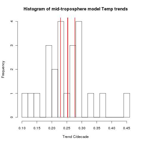
    However, it's clear to me now that this problem extends even to the analysis of the sample that they looked at. They list, in Table 1, the data series and their trends with standard error. The first 23 are models. In Figs 2 and 3 they show the model mean with error bars. I looked at the mid-trop (MT) set; in Table 2 they give the mean as 0.253, sd 0.012, and indeed, with error bars 0.024 that is what Fig 3 seems to show.


    So I plotted Table 1 as a histogram. Here's how it showed, with the mean and error bars from Table 2 MMH marked in red.


    The key thing to note is what James Annan also noted. The models are far more scattered than the supposed distribution indicates. The models themselves are significantly different from the model mean.

    Update: Of course, the error bars are for the mean, not the distribution. But the bars seem very tight. A simple se of the mean of the trends would be about 0.022. And that does not allow for the uncertainty of the trends themselves.

    Update 2: As Deep Climate points out below, that last update figure is wrong. A corrected figure is fairly close to what is in MMH's table.
    However, Steve McIntyre says that the right figure to use is the within-groups variance - some average of the se's of the trends of each model. That does seem to be the basis for their figure. I think both should be used, which would increase the bound by a factor of about sqrt(2).


    Wednesday, August 4, 2010

    Reduction of station numbers in GHCN


    As I noted in the previous post, a new post has appeared at WUWT  which talks a lot about the reduction in station numbers in GHCN that occurred between about 1990 to present. This post is based on a paper by Ross McKitrick.

    The stream of articles that advance various theories about this reduction don't take proper account of the way GHCN was actually compiled. It was initially a historical process, where in the early 90's with grant funding people gathered together batches of historic records, recently digitised, into a database. After V2 came out, in 1997, at some stage NOAA undertook the task of continuing monthly updates from CLIMAT forms. This made it, for the first time, a recurrent process.

    Update: Carrot Eater, in comments, has pointed to a very useful and relevant paper by Peterson, Dann and Phil Jones. As he says, the process wasn't quite as I've surmised. I should also have included a reference to Peterson's overview paper.


    The big reduction followed changes of policy in going to a recurrent process. As a batch process, it didn't really matter if the geographic spread was uneven. If the records were available, they could be included. But as a recurrent process, it makes sense to spread the effort of updating reasonably evenly worldwide.

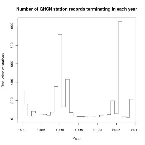
    If you look carefully at the time sequence of station terminations, it looks like this:


    It clearly consisted of a few major culling events. In the next table, the years with more than 100 stations ending are shown with a breakdown by country:


    This makes the pattern clear. Australia, Canada, China, S Africa, Turkey and USA had been overrepresented, and were culled in specific events. Canada in 1989/90, Turkey and China 1990, S Africa 1991, Australia 1992 and the USA in 2004 and 2006. The case of the US is special, because the USHCN database is also used.

    So when it is said that the reductions produced a reduction in average altitude or latitude, that reflects the fact that some of these countries are relatively high, and are (mostly) from temperate latitudes.

    Of course, explaining how and why the reduction happened doesn't remove the possibility of biasing a trend estimate. That's another story.


    Tuesday, August 3, 2010

    GE visualisation of changes to GHCN stations 1990-2007

    At WUWT there is a post about Ross McKitrick's discussion of supposed defects in GHCN, focussing heavily on changes in the stations in the dataset between about 1990 and 2005+. So I've made some KMZ files so interested people can see in detail what those changes were.

    This post follows three recent previous posts here about KMZ files for GHCN type datasets:
    Briefly, a KMZ file is a compressed file of data which you can read into Google Earth. You can just click on the filename in a file browser, or use the GE open facility (or Ctrl-O). When you open it, you will see a subset of the GHCN stations marked with placers (pushpins). These show (when you get close) the station names, and indicate other properties thus:
    • Color - rural stations are green, urban yellow. Orange is a small town.
    • Size. Big pins have >50 yrs data. 70% pins have >20 yrs, and 40% have less.
    • Balloon - clicking on a station gives a balloon with several data items, including years of reporting.

    The files


    You can find the files on the data repository. They are in a zip file KMLGHCNends.zip which you can download (scroll down). The individual files are:
    • GHCN1900end.kmz, which has stations that dropped out of the database between 1991 and 2000
    • GHCN2000end.kmz, which has stations that dropped out of the database between 2001 and 2007
    • GHCN1900st.kmz, which has stations that were added between 1991 and 2000
    • GHCN2000st.kmz, which has stations that were added between 2001 and 2007
    There weren't many stations added, so you might want to skip the last two files.

    Below the jump, I'll add some still pictures from GE.


    Here are the US stations that were dropped from GHCN between 1991 and 2000:


    Australia was very densely represented pre-1990, so many did not continue:


    African stations in W Africa and S Africa were not continued:


    Arctic losses were not large:


    Europe lost a few stations, including a bunch of short-record ones in Yugoslavia


    Between 2001 and 2007 the big change was US numbers - tied in with the interaction with USHCN, which GISS incorporates separately.