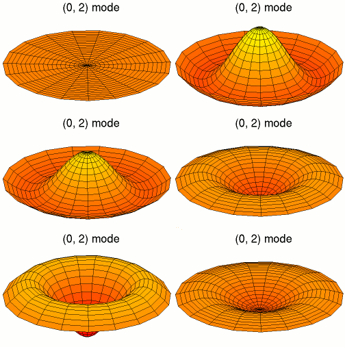
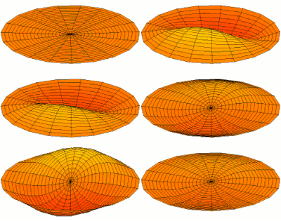
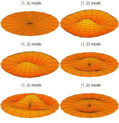
Chladni patterns are modes of oscillation, originally of a vibrating plate. Now people more often think of a drum membrane, which is a slightly different wave equation, but the idea, and patterns, are similar.
I must admit that I hadn't heard of Chladni before Hans Erren drew attention to them in Steve's first post. Some interesting history there. But I am familiar with the modes in question.
Steve thinks that if a Chladni pattern emerges, that somehow means that the result is showing that rather than the information about the climate pattern being sought, so the information content is reduced. I don't agree - there are reasons why the patterns arise, and they are just as informative in PCA as they are in wave studies. I'll try to show why.
Warning - mathematics (and \(\LaTeX\)) after the jump.
Resonance and wave equations
Resonance is familiar with acoustics. If you speak in the open air, your voice propagates away in all directions, attenuating without reflection or selective amplification. If you stand in a partly enclosed cavity, your voice is slightly louder in certain frequency bands. In a totally enclosed bare room, you hear a characteristic booming response - some frequencies are much louder.These are the ones that excite a resonant mode, in which the air oscillates, but the normal velocity at the boundary is zero. A 3D version of the modes of a vibrating stretched string, which has zero velocity at its ends.
The essential requirement is that the wave energy must be confined but not dissipated. That is why the resonance improves in deeper cavities, for example.
The wave equation for pressure, say, is (with c=speed of sound) $$\nabla^2 p = \frac{1}{c^2}\frac{\partial^2 p}{\partial t^2}$$ If you substitute a resonant mode \(p=P \sin(\omega t)\), then the equation is $$\nabla^2 P = -(\frac{\omega}{c})^2 P$$ P is the resonant mode, and so is an eigenvector of the Laplacian \(\nabla^2\). The resonant frequencies correspond to the eigenvalues.
For Chladni's plate the wave equation is more complicated, but the principle is the same.
Spatial autocorrelation.
Steve McI also described the simple Toeplitz autocorrelation coefficient matrix that you get in one dimension for a spatial model. With N+1 equally spaced points, the coefficients can be assumed to be powers of r - the correlation of adjacent sites. The matrix is: $$R = \left(\begin{array}{ccccc} 1 & r & r^2 & \ldots & r^N\\ r & 1 & r & r^2 & \ldots \\ r^2 & r & 1 & r & \ldots \\ \ldots & \ldots & \ldots & \ldots & \ldots\\ r^N & \ldots & r^2 & r & 1 \end{array}\right) $$ The Toeplitz property is that all terms on each diagonal are the same. This correlation matrix has a simple inverse: $$R^{-1} = \left(\begin{array}{ccccc} q & -qr & 0 & \ldots & 0\\ -qr & 2q-1 & -qr & 0 & \ldots \\ 0 & -qr & 2q-1 & -qr & \ldots \\ \ldots & \ldots & \ldots & \ldots & \ldots\\ 0 & \ldots & 0 & -qr & q \end{array}\right),\quad q=\frac{1}{1-r^2} $$ Still a Toeplitz matrix, almost, but also banded - tridiagonal. The deviation from Toeplitz is at the top left and bottom right corner terms.Relation to Laplacian and the wave equation
From the last equation, $$\begin{align} R^{-1} &= qr\left(\begin{array}{ccccc} 1/r & -1 & 0 & \ldots & 0\\ -1 & r+1/r & -1 & 0 & \ldots \\ 0 & -1 & r+1/r & -1 & \ldots \\ \ldots & \ldots & \ldots & \ldots & \ldots\\ 0 & \ldots & 0 & -1 & 1/r \end{array}\right) \\ &= qr\left(\begin{array}{ccccc} 1 & -1 & 0 & \ldots & 0\\ -1 & 2 & -1 & 0 & \ldots \\ 0 & -1 & 2 & -1 & \ldots \\ \ldots & \ldots & \ldots & \ldots & \ldots\\ 0 & \ldots & 0 & -1 & 1 \end{array}\right) + q(1-r)^2 \left(\begin{array}{ccccc} 1/(1+r^2) & 0 & 0 & \ldots & 0\\ 0 & 1 & 0 & 0 & \ldots \\ 0 & 0 & 1 & 0 & \ldots \\ \ldots & \ldots & \ldots & \ldots & \ldots\\ 0 & \ldots & 0 & 0 & 1/(1+r^2) \end{array}\right) \end{align} $$ If you remember finite differences, the first matrix is just the negative of the second difference operator, corresponding to the 1D Laplacian. And the second is almost a multiple of the identity, and is small if r is close to 1.That's the key to the connection between Chladni patterns and the autocorrelation matrix R. The inverse of R and the Laplacian of the wave equation differ by close to a multiple of the identity, which means they have almost the same eigenvectors. And the eigenvectors of R and \(R^{-1}\) are the same. R is symmetric and positive definite.
Subtle differences
Well, an unsubtle difference is that Chladni oatterns are not 1D. But the same reasoning works - it's too messy to set out here.The subtler difference is that the diagonal correction is not quite Toeplitz. That relates to the notion of boundary conditions for the wave equation, which is indeed critical for resonance.
At this stage I'll have to just arm-wave on that - it does in fact give the zero normal boundary condition, which is sufficient for resonance.
Conclusion
The same mathematics that gives Chladni for the wave equations gives similar eigenvectors for the spatially autocorrelated matrix. It isn't a spurious consequence. Consequently their appearance in, say, Steig et al 2009 doesn't mean that the PC's are "just Chladni" any more than they are just autocorrelation. Spatial autocorrelation is an essential part of the results, and the Chladni patterns reflect that.I think that's enough heavy maths for now - I could later go more into the properties of Chladni patterns, and in particular into the implications for eigenvalue pairing (for PCs) which SM criticised in Steig et al. That would generate pretty pictures.
Meanwhile, I'll just relay these pictures of resonant modes from Wikipedia where more Chladni patterns on the disc and sphere can be found.

| 
| 
|

| 
| 
|


